In the previous entry, the basis for classifying our test images was the distance from the training images on the color versus shape plot. What I will be showing you now is the use of neural networks to actually train the computer in identifying the characteristics that I need from the set of images. The term "training" for the previous entry was loosely used, as I simply measured two parameters on the two sets of images and used them as reference points.
The artificial neural network toolbox of Scilab accepts different parameters for the training: number of iterations, tolerance, and learning rate.
Using the same set of data obtained by characterizing the "shape" and "color" of the petals of the blue plumbago (Plumbago auriculata) and galphimia vine (Galphimia gracilis), the following output was given by the ann_FF_run() function:
first sample: 0.5002511
second sample: 0.5023937
third sample: 0.5002258
parameters:
learning rate: 2.5
tolerance: 1
iterations: 700
If you'd remember, the first and third samples are of the blue plumbago and the second one is from a galphimia vine. The results indicate that with the given parameters, the computer was able to determine which of them come from a certain type of plant. Although the value given for the first and second differ only by as much as 0.002, we can say that the output is reliable, as the difference between the first and the third vary only by around 0.000025. The first difference is almost 100 times than that of the second.
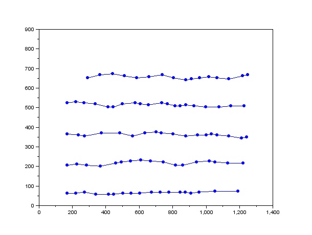
I tried to vary the number of iterations that the ANN toolbox would use, and found this result:
Figure 1. Plot of output versus the number of iterations for the training process. the blue triangle and star correspond to the first and third sample respectively and the yellow circle correspond to the second sample.
You'll see that at some point the outputs are higher for the blue samples than the yellow sample, and in the other the opposite is observed. For this to be applied on a completely unknown sample, we must first compare it to test sets to have a reference.
For this activity, I will give myself a grade of 10/10.
How do we classify plants? We usually look at the shapes of their leaves or observe the color of their fruits. As I recall from my previous Biology classes, the leaves vary from one plant to another, may it be the base, apex, or outline of the leaves. Also, we expect that the color of the fruit is the same as the color of the flower. Fruits with a dark red or violet to dark violet colors are rich in anthocyanin, which increases the amount of anti-oxidants in our body. So the next time you buy apples, choose only those with a dark red color. Those that have a red with yellow patches tend to be older and have lost their anthocyanin.
Anyway, I'm a physicist so I might be wrong :D What I'll be discussing in this blog is recognizing patterns from images. I captured photos of two types of flowers in UP Diliman:
Figure 1. Blue plumbago (Plumbago auriculata)
Figure 2. Galphimia vine (Galphimia gracilis)
I didn't know what these flowers are. I had to post it on my Facebook account and wait for someone to name them. Luckily, my friend Frances was familiar with these flowers! *phew* It saved me a lot of time looking for their names.
My goal is to have a measure on these petals in such a way that when I have one of them, I'll be able to tell what flower it is. But instead of picking the flowers and tearing the leaves apart, I just took photos of them at different angles and lighting.
Figure 3. Training set for the blue plumbago
Figure 4. Training set for the galphimia vine
No, I really can't pull out the petals even for the sake of the activity. I used GIMP to remove the petals from the flowers to have 10 training images for both flowers. It's difficult to use image segmentation based on the colors, as it will locate the entire flower from the image. Brute force was needed to have training sets.
I characterized the petals according to:
SHAPE - well not actually shape, as I found no means to measure the shape or determine the type of its base, apex, or what. I measured the ratio of the area of the blob (which is simply the number of nonzero pixels) to the area of the region enclosing the blob (from the AnalyzeBlob function of Scilab, I got the coordinates of the bounding box). Figure 5 below illustrates the regions of interest for both type of flowers. As you would see, the blue plumbago occupies more region on the bounding box than the galphimia vine because it is more round. The epithet auriculata pertains to the ear-like feature of the petal [1]. The petal of the galphimia vine has a pointed base, allowing more black pixels to occupy the bounding box.
COLOR - from the normalized chromaticity coordinates, I measured the distance of each data point (on the NCC) from the origin and summed them all up. I know this is a weird method, but then again I can't think of any other way to have a measure of the color.
Figure 5. Estimate of the shape of the two types of petals
Figure 6. Quantifying the values from the normalized
chromaticity coordinates
From these classifiers, I plotted the training sets:
Figure 7. Locating the training sets on the color versus shape plot. Blue dots indicate the training images
for the blue plumbago flowers, yellow dots indicate those of the galphimia vine flowers.
Now that I have a clustered plot (the training sets are quite grouped close to each other), I will now try to locate these three test petals:
Figure 8. Test images. The symbols below indicate the legend for the next plot.
Using the same measures for the shape and color:
Figure 9. Locating the test images.
Based on Figure 9, by visual inspection, we can say that the two blue plumbago test petals are closer to the majority of the blue dots. Similarly, the test petal for the galphimia vine petal was closer to the yellow dots. Using simple distance measurements:
Table 1. Distance of the test images from the training sets
You'll see that both the first and third test images (both blue plumbago petals) have smaller distance from the blue compared to the yellow, while the second image (galphimia vine petal) has a smaller distance from the yellow compared to the blue. This shows that using the two classification schemes, I was able to determine what flower our test images come from.
For this activity, I will give myself a grade of 12/10.
EDITED:
I tried another classifier for the shape:
Figure 10. Ratio of the longest segment to the area of the petal
Then ended up with this:
Figure 11. Plot of "color" versus "shape" using the measurement from Figure 9.
The results are quite similar:
References:
[1] Harrison, Lorraine (2012). RHS Latin for gardeners. United Kingdom: Mitchell Beazley.
The file size of images can be reduced by performing image compression. When we capture images using our cameras, they are usually compressed immediately as JPEG files. Most digital single lens reflex cameras (DSLR's for short) allows the user to retain all the information received by the camera sensor (either CMOS or CCD) by providing a raw image. A high resolution image from my DSLR, which is in JPEG has a typical size of 4 to 6 MB. At the same time, a 20 to 40 MB raw file is saved. Discrete cosine transform (which I have mentioned way back) is performed on the image to achieve a smaller file size.
Image compression can also be performed using the concept of principal components. An image can be decomposed into a set of principal components. To visualize how it works, think of a point in a 3-dimensional space. Its distance from the origin can be described by its location along the x-, y-, and z-axis. Furthermore, if we have an multi-dimensional space, the location can be described with respect to the vectors that are orthogonal with each other. However, some of these vectors constitute a small portion on the measurement of the location of one point on the multi-dimensional space. If we neglect them, we can still be able to have a rough estimate of the location.
The same goes for image compression. This image:
Figure 1: Image that will be used for compression. (Photo credit: Norman Mascariñas)
Figure 2. Gray scale image of the red component of Figure 1
after using the pca() function of Scilab, produces a set of images like this (obtained from facpr of the function pca):
Figure 3: Principal components
The original image (800x500 pixels) was split into 10x10 sub-images. This is why we have principal components that are 10x10 pixels each. As mentioned earlier, these components (the eigenvectors of the image) will become the bases for the reconstruction of each sub-image. You will see in Figure 3that the first component (top left) have larger clustering than the other ones, with the last component (bottom right) having the smallest or finest pixels. Choosing the number of principal components depends on the contribution of each of them (which can be obtained from lambda of the function pca). This can be shown as:
Figure 4. Cumulative contribution of the components
You'll see that there is a steep increase in the contribution from the first four components. This means that we adding one component at a time will give a noticeable change in the overall reconstruction of the image. Beyond the 40th component, the contribution no longer changes, which gives us an idea that the reconstruction will not have any difference, whatever number of components we select.
To reconstruct the image, I used the first M components and get the corresponding values in comprinc for each sub-image. The function pca() computes individually per sub-image, so we need to retrieve the "intensity" of each component for every sub-image.
Figure 5. Comparison of image reconstruction, with the number beside each indicating the number of
components used for reconstruction
As expected, the first few reconstructions are more "pixelated", meaning they look like they have chunks of pixels.. Zooming in on the first reconstruction:
Figure 6. Reconstruction using only the first component
It really is a bad reconstruction, and looks like the usual images compressed using DCT at low compression rate. Increasing the number of components, as seen in Figure 5, produces a sharper and smoother image.
Figure 7. Reconstruction with 20 components
Figure 8. Reconstruction with 90 components
Comparing Figures 7 and 8, we see that there are no visible differences between the two. With this, we can just select the right number of component, which would roughly give around 99% of the image. Both of them (Figures 7 and 8) have cumulative contributions greater than 99%.
For this activity, I will give myself a grade of 10/10.
Reference:
A13-Image compression. M. Soriano. 2013
Figure 1. Can you guess what music is this? Clue: food!
I won't be naming this score sheet at the moment. I got this score sheet from www.flutetunes.com. For now, I'll discuss how to process this image in a way that the computer will be able to read each note, and hopefully with the corresponding duration of the tone. I selected this piece because first this is a Filipino song (another clue!) and second is that this is in C major, which reduces the complexity of processing the score sheet. The problem with those in other majors is that the natural symbol is often added at certain notes to remove the flat or sharp. Also, I chose this music because there are no rests, which have a lot of varieties in appearances, depending on the duration of the rest. To further simplify the activity, I removed the clef and the time signature:
Figure 2. Same score sheet but with fewer symbols.
First, I try to locate the position of the staves:
Figure 3. Plot of the line scan at the 531th column. This column was chosen
because there will be no intersection with other symbols along the scan.
Figure 3 looks the same as the staves because the plot was made to connect successive points. Since the locations look like Dirac deltas that are separated by around 20 pixels, using only dots or circles to denote the location of the peaks at the cross section would look flat:
Figure 4. Plot of the line scan at the 531th column. Similar to the previous, but
scaling was performed to make it look better.
Now that we have the locations of each line for all the staves. we use them to approximate the position of the notes. But we'll leave that aside.
To simulate the music from the score sheet, we need to determine not only the note but also the duration of the tone. In the score sheet above, there are half notes, quarter notes, and one-eight notes. Also, there are dotted notes, with the dot indicating a duration for the note that is 1.5 times the original duration of the note.
I was able to differentiate the half notes and quarter notes using edge detection and template matching. I selected the round part of a quarter note and obtained its negative, then performed edge detection.
Figure 5. Left: original "note", center: negative of the previous.
right: image for template matching.
The image on the right of Figure 5 was added to a black image with the same size as the image of the score sheet. I'm not going to display it here because the score sheet has a dimension of 807x1362 pixels (row x column), and the image containing the trace of the note has a dimension of 76x17 pixels, making the final image for the template a black image with a small white smudge at the center.
I also obtained the negative of the score sheet:
Figure 6. Negative of the image in Figure 2.
Using template matching using cross correlation and thresholding, as performed in one of my previous entries, I was able to get the following image:
Figure 7. Result of template matching and thresholding.
Comparing Figures 6 and 7, you'll see that the larger blobs correspond to half notes while the smaller ones correspond to the quarter and one-eight notes.
HMMM. For now i'll be neglecting the difference between the quarter note and one-eight note, as well as the dot. If time permits, I'll be working on these things.
After much deliberation on how to trace the notes that belong to the same staff, I've become successful! Yeah!
Figure 8. Location of the centroid of the notes. The lines connecting
the dots indicate that they are on the same staff.
Impressive isn't it? For me it is. After all, I've spent at least 4 days thinking about this. By locating the 5 lines on the series of staves, I scanned through the image from the first row to the row between the first E4 to the second F5, then to the row between the second E4 to the third F5, and so on. In Figure 9 below, the red dots indicate where the scanning through the rows per staff will be limited.
Figure 9. Separation of the staves.
Oh, and by the way, the points in Figure 8 representing the centroid of the notes was determined using the combination of the functions SearchBlobs() and AnalyzeBlobs(). This also allowed me to determine which note would come first for each of the staves.
At the moment, I'm already able to tell which line or space does one note fall on. To know the duration of the note, I used a threshold value different from Figure 7:
Figure 10. Different thresholding
You'll see, by comparing with Figure 2, the large chunks of blob correspond to the half notes while the smaller and diffused speckles correspond to quarter notes and eight notes. I scanned around the centroids, which I computed previously, then count how many non-zero pixels are there.
Figure 11. Area measurement of each blob.
Good thing There are extreme values of the number of pixels for the half notes and quarter notes. I assigned the blobs with more than 300 pixels to be half notes while the rest are considered to be quarter notes. Sorry guys, I'm taking a risk here by having some notes take a longer time than what was indicated in the score sheet. But then again, if we have the half note take a duration of 0.5 second, what huge difference would it make to have all the quarter notes and one-eight notes last for 0.25 second? At the same time, I also neglected the presence of dots beside the notes. Hopefully we would still hear a good music. We'll see later :D or hear.
So here it is, the plot of the locations of the centroid on the image, with the red stars representing the half notes and the blue dots representing the quarter notes and one-eight notes:
Figure 12. Location of the notes on the image. Red stars: half notes; blue dots: quarter notes and one-eight notes
After three days, Scilab was able to finish performing the song. YES THREE DAYS. I don't know why it took Scilab that long. Maybe I should have deleted the other variables to empty up the memory of the computer. And because of that I was not able to do my other blog activities. Oh well, have fun listening to the song!
For this activity, I would give myself a grade of 12/10 because I used different techniques:
edge detection - which is actually a weird but novel approach, i think. this is to pick up only the notes
template matching - locate the notes based on the reconstructed edge of the note
blob analysis - finding the centroid of the notes
morphological operations - determine the duration of the note. analysis of the size allowed me to determine which are the half notes and which are different
this one is actually not a technique, but it was fun doing the activity by analyzing the entire image, and not by first dissecting it to different staves. what's cool about this is that the program then analyzes the score sheet from the first measure through the final measure, all found on the same image.
And I'm also proud of my work since I did this for two agonizing weeks. Plus the song is very...nationalistic? hahaha. :)
References:
1. A12 - Playing notes by image processing. M. Soriano. 2013.