Tuesday, August 20, 2013

Application of Binary Operations

In this activity, we try to identify the areas of blobs in an image and locate which of them are "abnormal", based on the mean and the standard deviation of the areas. This method is important in biomedical imaging, particularly in identifying cancer cells.

Our sample image, Figure 1, contains numerous circular shapes with uniform areas. With visual inspection, we identify the abnormal cells to be the ones enclosed with a red rectangular shape in Figure 2.
Figure 1. Collection of "cells" with randomly placed "cancer cells"

Figure 2. Identified "cancer cells"

Before we can locate these cancer cells, we first need to "calibrate" our detecting system using a set of normal cells. We were given the following image as a basis for measuring the mean area of the cells:

Figure 3. Collection of "normal cells" for calibration

This image was split into smaller images, and each of them were converted to black and white.
Figure 4. Conversion of image segment to black and white.

Reducing the image to black and white produces an image with random white spots, which are part of the background but are above the threshold value set using the function im2bw(). Since it would be difficult to determine the exact value for the threshold in order to eliminate the noise, we need to have a system that would remove these spots. Morphological operations will allow removal of these random spots by locating the shapes of specific sizes and shapes and retaining only those that will satisfy the structuring element. The function OpenImage(im, se) of Scilab performs an erosion of the image im using the the structuring element se. Afterwards, it performs a dilation on the image using the same structuring element. The function CloseImage(), also a morphological operation, is similar to OpenImage(), but instead performs dilation before erosion.

Using the function CreateStructureElement(), I created a circular structuring element with a dimension of 11x11 pixels. With OpenImage(), the spots were removed:

Figure 5. Noise reduction using OpenImage()

You would also notice that the cells on the image at the right portion of Figure 5 have different gray levels. The cells were labeled using the function SearchBlobs(), which identifies continuous portions on the image. The clump of cells at the right-center only has 1 value for the gray level, meaning the function identifies it as a single cell. This would cause problems later in the process of measuring the mean area of the cells. 

Performing these operations on all the subimages, I now have the following: 

Figure 6. Noise reduction for all the subimages

Figure 7 below shows that we can isolate each blob. From these segments, we can have a measure of the area of the cell, which is simply the number of pixels having 1 as a value.

Figure 7. Isolation of different blobs

Using histplot(), I obtained a histogram of the measurements of the area for all the blobs.
Figure 8. Histogram of the area measurements

There are extreme values for the area with low frequencies, all located beyond the 1000-pixel mark. These measurements arise from the cells that overlap each other and formed a large blob. We neglect these values since they are obviously not the values that we need to approximate for the cell sizes. Selecting only the values for area below 900 pixels and above 300 pixels. The latter criterion was imposed because there are cells located at the boundaries of the image, which constitute the distribution at the left end of the histogram. Using these values, the cell size was found to be 507.23 pixels with a standard deviation of 90.44 pixels.

With these measurements, I was able to locate the cancer cells from the given image:
Figure 9. Identified cancer cells

There was an additional trick however, aside from using the mean and standard deviation values for the area. After I have located the blobs with areas outside the acceptable values, I performed another OpenImage() step, but with a much larger structure element. I used a circular structure element with a radius of 15 pixels. Without this step, the program will retain the blobs that represent overlapping cells, which actually have areas larger than the acceptable value. However, as mentioned previously, these are not the cells that we want to locate. With this, we now only have the cancer cells.

For this activity, I'll be giving myself a grade of 10/10 for accomplishing the activity properly.

Reference
A11 - Application of Binary Operations: Blob Analysis activity manual. M Soriano. 2013.


Sunday, August 11, 2013

Enhancement in the Frequency Domain

In this activity, our goal is to eliminate unwanted information in an image by manipulating in the frequency domain. But first, we investigate what the frequency domain looks like for different types of images. 

Two dots (1x1 pixel each) was placed equidistant from the center of the 128x128 pixel image. These dots represent a pair of Dirac deltas, which is the Fourier transform of the sine function. The spacing between the two Dirac deltas is twice the frequency of the sine function. Using fft2() on the images containing two Dirac deltas (images at the upper part of Figure 1) produces a matrix containing the inverse Fourier transform. That is why the images at the lower part of the same figure show sine functions of increasing frequency (smaller gap between successive bands) as the spacing between the Dirac deltas is increased.

Figure 1. Pair of Dirac deltas and corresponding inverse Fourier transforms.

In the fo


Sunday, July 21, 2013

Fourier transforms

In this exercise, we worked with Fourier transforms and convolution of images using the built-in "Fast Fourier" transform function in Scilab. Fourier transforming a signal will give us a representation of the distribution of the frequencies present in the said signal. A signal can be decomposed into a set of sines and cosines, with amplitude and frequencies depending on the computation of the discrete Fourier transform. 

An image is basically a signal, since it is a collection of information stored in a series of pixels. In photography, for example, information (color, brightness, etc) is transferred from the subject to the pixels of the camera. Depending on the properties of a portion of the subject, the region of the camera's sensor will store a corresponding signal. After processing these signals, we are able to view the subject in a photograph, which would hopefully be as colorful (or vibrant or whatever) as the subject.

Anyways, so there. Scilab has the function fft() and fft2() to perform a discrete Fourier transform, for one-dimensional and two-dimentional signal respectively. In our case, since we're dealing with images, which are 2D, we will be using fft2. Additionally, these two functions also perform the inverse Fourier transform, which is quite handy.


Figure 1. Transformation of two images to frequency space and back to the original.

Side note: It took me so long to finish this exercise because I can't figure out the problems in my Scilab code. Actually there were no errors. It's just that I didn't use the function mat2gray(), which converts a matrix (containing the information from the Fourier transformed image) to a grayscale image. Meryl told me to add this function to create the desired image of the Fourier transform and for the other images. Without her suggestion, I wouldn't be able to do the entire exercise. Seriously hahaha.


Figure 2. Conversion of the matrix to an image using mat2gray()


Going back to Figure 1, after performing Fourier transform, we still need to use the function fftshift(). As seen in the second column of Figure 1, the white regions, which contain the information from the Fourier transform, are distributed to the four corners of the image. Using fftshift() forces these white regions to be placed at the center of the image. As seen on the Fourier transform of the circular aperture, the result is an Airy pattern. Also, the inverse Fourier transform of the Fourier transform of the image containing the letter "A" is inverted, as opposed to the original image.

Simulation of an imaging device

Due to the finite sizes of the optical components of an imaging device, a photograph can have a lot of differences from the subject. The quality of a photograph differs from the subject as a result of the latter's convolution with the transfer function of the imaging device. A set of lenses with large diameters will produce sharper images compared to small diameters, as more rays from the original image will be allowed to pass through, which will then contribute to a wider range of information.

If we have a convolution of two functions, we can obtain the result from the multiplication of the Fourier transform of the subject and the Fourier transform of an imaging device. Afterwards, we perform inverse Fourier transform on the product. 

In an optical system, lenses automatically perform Fourier transform on an image [1]. We can think of it as the aperture being already at the Fourier plane, and we simply multiply it with the Fourier transform of the image. 


Figure 3. Simulation of an imaging device of different aperture diameters.

As expected, those with smaller diameters produced blurred images compared to those with larger diameters.

Template matching

We can also perform template matching using correlation. Similar with the previous one, we work with the Fourier transforms of two images. In this part, we use an image containing the text:
THE RAIN IN SPAIN STAYS MAINLY IN THE PLAIN
and a template image, of the same size as the first image, containing only the letter "A", which is what we need. Using correlation, we can determine the location of the letter "A" (from the template) on the first image. For both images, the font sizes and styles are similar. 

However, instead of multiplying the Fourier transforms right away, we first perform complex conjugation (using the function conj() ) on the template image. 

Figure 4. Text image and template image

Using the described method, I got this image:

Figure 5. Correlated image

By correlating the two images, the peaks (indicated by the bright spots) occurred at the locations where A is found on the text image. As you can see, the letter A is highly smeared on every point on the letters from the text image, causing the blur on the correlated image. At the regions where the template smeared exactly on the same letter, bright spots formed, indicating a strong correlation.

Performing thresholding on Figure 5, I was able to locate the bright spots:

Figure 6. Thresholding of the correlated image

This was produced using the function SegmentByThreshold(), with the threshold set to 0.8. These bright spots are the locations of the letter A in the text image. 

Edge Detection

Edge detection can also be performed by convolving an image with a 3x3 matrix of a specific pattern. The matrices that were created consist of elements having a sum of zero. In the following image, we see each matrix, followed by a 128x128 pixel image with the matrix at the center, and the resulting image after convolving with the original image (as seen in Figure 3).

Figure 7. Convolution of the Fourier transform of the original image and a 3x3 matrix.

The first matrix was able to detect the horizontal edges of the image containing the word "VIP" while the second matrix was able to detect the vertical edges. In addition, the diagonal lines were also detected by the second matrix since these lines are composed of short vertical lines. The final matrix was able to detect both the vertical and horizontal edges on the original image.

For this activity, I would give myself a grade of 10 since I was able to perform the activity correctly.

Reference
Activity 7- Fourier transform model of image transformation. M. Soriano. 2013.


Thursday, July 4, 2013

Revealing dark secrets using Histogram manipulation

Or not.

In this activity, I tried to manipulate the histogram of a dark image to enhance the contrast. This allows the details in the dark regions of the image to appear.

Wait a second, what exactly is a histogram?

I mentioned the term previously but I haven't discussed it yet. My bad.

A histogram is a representation of the occurrences of data points. In image processing, we are concerned with the brightness histogram of an image. Each pixel in the image will have a specific brightness, and thus creating a histogram of the image will display the frequency of each level of brightness (from 0 to 255). In brightness histograms, we will not be dealing with the location of the points containing these levels of brightness. Since it displays the frequency of each value, it can also be viewed as a probability distribution. Hereafter, histogram and/or probability distribution function (PDF) will be used instead of brightness histogram for simplicity.

For the activity, we will be dealing with grayscale images. We expect that for a dark image, the histogram will be skewed towards the far left, near the zero value of intensity.

So before we proceed, here's a summary of the activity:


Figure 1. Flowchart

To be able to understand this, I'll give an example.

In this picture, (I can't remember who took this photo, I just found this somewhere in my astrophoto folders), the small amount of light makes it difficult to see a lot of details at the bottom part. Well, the CS basketball court would be the best place to set up a telescope because there are no lamps nearby (except those around NIP) and it's safe. So if you want to observe the night sky with a telescope, this is one of the nicest place in UP for observation. :D

In any case, at the lower part of the image, I'm there preparing the telescope. And there are bags nearby. But since it's dark, it's difficult to notice.

Figure 2. Image to be manipulated

Converting this to grayscale with Scilab:

Figure 3. Grayscale version of Figure 2

Why do we need to convert it? This makes it simpler, as we only need to manipulate the brightness of the image. Ma'am Soriano told us that we can split the colored image into red, green, and blue channels and individually convert them to grayscale. With these grayscaled channels, the brightness of all the three colors can be manipulated. How? I don't know yet, Ma'am Soriano is yet to teach that method in their Applied Physics 187 class. TOO BAD, I don't have Applied Physics 187.

Here's the normalized histogram/PDF of Figure 3:
Figure 4. Normalized histogram of Figure 3. The frequencies of the intensities are divided by the total number of pixels in the image to normalize the histogram.

As you can see, the frequencies are high only at the 0-50 intensity levels. The image really is dark. So to enhance it, we introduce the concept of cumulative distribution function (CDF). Simply put, it is obtained by adding the normalized frequency at each value (in this case the intensity/ brightness level). The CDF of Figure 4 is:
Figure 5. Cumulative distribution function of the histogram in Figure 4.

We need another CDF, which is what we want to achieve for the original image. First, we use a linear CDF as our target CDF. For all brightness level in the image, there exists a CDF value in Figure 5. We then find this CDF value on the second CDF and determine the corresponding brightness level.


Figure 6. Obtaining the new pixel value using the original CDF (left) and the desired CDF (right)

If it's hard to process what I said in the previous paragraph, maybe Figure 6 can help. This shows that all pixels in the grayscale image with 30 as the brightness level will now have an intensity of 210. The final image, after applying this transformation is:

Figure 7. Enhanced image using a linear CDF

Works like magic. Haha. There, you can see me clearly and also my friend's bag. In addition, the letters from the word "NATIONAL" became more visible. You can also see the three-point "line" and the difference in the type/color of paint between the parts of the basketball court.

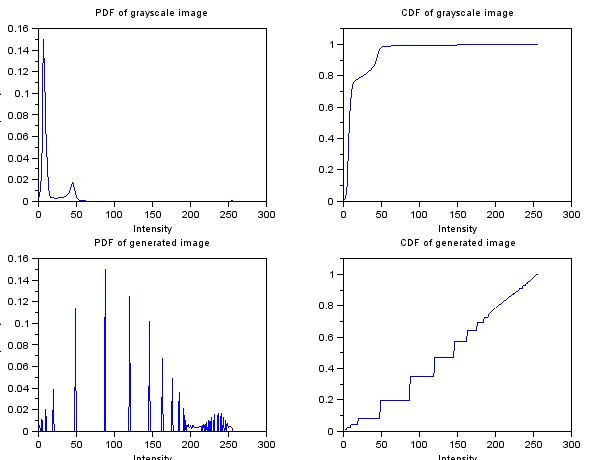
Here are the PDF's and CDF's of the grayscale and generated image:
Figure 8. Histogram and CDF of the image before (top) and after (bottom)

The spread of the histogram, after linearization of the CDF, became wider across 0 to 255. Also, the plot at the lower right of Figure 8 shows the CDF of the new image, which shows that indeed the CDF became linearized.

I also tried using a Gaussian distribution with varying standard deviation to manipulate the image. And here are the generated image, followed by the PDF's and CDF's.


Figure 9. Enhanced grayscale image. Standard deviation of 20 brightness levels were used for the Gaussian distribution, centered at 255/2.

Figure 10. Histogram and CDF of the image before (top) and after (bottom)

Figure 11. Enhanced grayscale image. Standard deviation of 40 brightness levels were used for the Gaussian distribution, centered at 255/2.

Figure 12. Histogram and CDF of the image before (top) and after (bottom)

You can see that the transitions between different objects in Figure 11 are more pronounced. This is because the brightness levels near zero and 255 have more frequency, as seen in the lower left plot in Figure 12, compared to that in Figure 10. Since the brightness levels peak at the mean brightness level and the distribution is narrow (standard deviation of 20 levels). Going back to the original concept, what we wanted was a histogram with values scattered from 0 to 255 right? We weren't able to see details in Figure 3 because its histogram is skewed towards zero. Even though the image became brighter in Figure 9, the distinctions between adjacent objects are not clear. With Figure 11, we obtained a relatively better image.


Let's use another image!

Figure 13. New image to be manipulated.


I took this image last February at the PAGASA Observatory in UP Diliman. The kids in the photo were having a field trip, waiting for the sun to set. During that night, they were able to spot Jupiter using the 45cm telescope of PAGASA. And here is its grayscaled version:

Figure 14. Grayscale version of Figure 13

Applying the same linear CDF, I obtained this image, followed by the original and resulting histograms and CDF's:

Figure 15. Resulting image after using a linear CDF


Figure 14. Histogram and CDF of the image before (top) and after (bottom)

Surprisingly, the enhanced image showed the shadow of the kids produced by the setting sun. The details of the plants, bushes, and trees appeared, as well as those on the building at the left (National Institute of Molecular Biology Building) and at the right (Kamia Residence Hall, I guess?). 

It really worked like magic haha. 

I also tried reproducing Figure 14 with GIMP using the Curves function under the Color Menu:

Figure 15. Enhancing the image in Figure 14 using GIMP.

Figure 16. Resulting image from GIMP

Figure 17. Histogram of Figure 16

With GIMP, I was able to make the histogram distributed over all the brightness levels, which is somehow similar to the lower left plot in Figure 14.

Out of 10, I would give myself a grade of 10 since I performed all the tasks well. Without Alix, I could not have done this activity. haha. At first, I manipulated the image pixel by pixel with the use of loop within a loop. It took an eternity to finish running, and produced nothing. Then she approached me and gave an overview of how she performed the manipulation. She taught me how to use the find() function properly. What I had in mind at first was to look for the pixel coordinates with certain brightness levels and collect their indices. She told me that I can just call the indices directly instead of storing them by appending the find() function to the matrix:
imgray2(find(imgray1==0)) = 255;
This line, for example, uses two matrices of equal dimensions. The first one, imgray1, contains the brightness levels of all the pixels from an image. With find(imgray1==0), the indices of all black pixels will be collected. putting that inside imgray2() calls these indices from the second matrix, and then we assign them with a value of 255. Creating an image from imgray2, we will see that it will be the same as the original image, only that the black pixels from the original image will become white.

So there you have it. manipulation of images using histograms. Hope you enjoyed it. :D

References:
[1]. Soriano, M. Applied Physics 186 activity manual - enhancement by histogram manipulation.


Tuesday, June 25, 2013

Pizzas and Area estimation of images

Last time, we tried to manipulate images by converting them to black and white and grayscale. These methods are helpful in measuring area covered by a region in an image. By having a "binary" image, that is, black and white, we will be able to represent the region that we want to observe in a manner that it becomes distinct from the background.

Once we have selected the region of interest, we will slice like a pizza!
Yummy! [1]

Any shape can be divided into several slices, such as in the following image:

Figure 1: Map of the United States of America. Or better yet, United Slices of America. [2]

By separating them into smaller triangles/ slices of pizza, we can approximate the area of the entire region by simply adding the area of all the triangles. But it would be troublesome to have weird shapes that will not provide us simple triangular shapes, as what you might see at the upper right part of Figure 1. If we were to measure such a region, we should segment it not just radially. Can't imagine how to solve it? Me neither. Well, not for now. Maybe next time. :P

So here, we will be limited to the application on simple shapes generated using Paint. Why Paint? For one, I don't have Photoshop right now. Another is that GIMP can't produce shapes. And another reason is that Paint can provide the dimensions of the shape that I'm creating. Well, Paint gives the length and width of the rectangular region immediately around the shape, which is what I'm after. Using these measurements, I'm able to compute for the actual size of the shape. With Scilab, I was able to compute for the area of the image by following this flowchart:

Figure 2: Flowchart of measuring the area of a shape

I tested the code that I've written on Scilab on a circle with a diameter of 300 pixels. Also, I tried placing the circle on different locations on the image to see if it would matter (which probably won't).
Figure 3. Circles with diameters of 300 pixels on a 500x500 pixel image. As will be used in the following table, the images are labeled according to their location: (a) center, (b) upper left, (c) lower left, and (d) bottom.

In Figure 3d, the circle is tangent with the border of the image, making the outline of the circle discontinuous in a sense.

Table 1. Actual and measured area of a circular region on an image

Yes, as expected, placing the circle away from the center will not give a difference on the area measured by the code. A small difference was observed on Figure 3d. When I was doing that image on Paint, I simply dragged the circle towards the edge of the image. Perhaps I did not notice that some parts of the circle went outside the image.

Or maybe it was due to the connection at the edge of the image. So I went on investigating about it by creating this image:

Figure 4. Semicircle with diameter of 300 pixels on a 500x500 pixel image

This image was also constructed using Paint. There was a 10.97% difference from the actual area of 35342 square pixels when the area was approximated using the Scilab code. Why is there a large discrepancy? I figured out that the edge() function was not able to detect the flat side of the semicircle positioned on the boundary of the image. To be sure, I plotted the points determined by the edge() function to be the edge of the white shape:

Figure 5. Location of the points determined by the edge() function to be the boundary of the semicircle that has a diameter of 300 pixels.

In Figure 5, the lines connect all the points on the edge. Seeing that there is a low density of lines at the upper portion, there should be a small number of edge points on that part. Also, even after zooming in at the upper boundary, there were no distinct connection of lines. With that being said, the code perhaps divided the semicircle to thin slices of pizza at the bottom part. At the upper portion, it created only one triangle with one vertex at the centroid of the semicircle, and the other two vertices at the right and left corner of the flat side. Having large slices of pizzas will decrease the precision of the approximation.


Application
Our house is located on a trapezoidal lot, which makes it difficult for me to describe the dimensions of our lot whenever my friends ask about it. With the help of Google maps, I was able to capture an image of our residential area:
Figure 6. Image of our residential area [3]

I saved a 941x552 square pixel image of this using the built-in Snipping Tool of Windows 7. From Paint, I was able to determine the ratio of meters to pixels by drawing a line over the scale bar. A ten meter distance on the image corresponds to a 77 pixels distance on the image.

Have you guessed where our house is? Of coures not. XD So here it is, with the lot covered by a red trapezod:
Figure 7. Our lot marked by the red trapezoid

Figure 8. Conversion of Figure 6 to black and white

Using the same code, the area was estimated to be 37776 square pixels, which would correspond to 637 square meters. Again, with Paint, I estimated the area of the trapezoid, assuming that the two bases (lower left and upper right edges) are parallel to each other. With that method, I measured the area to be 36206 square pixels, resulting to a 4.33 percent difference with the previous value.

How should I measure the actual value?

Mothers know best.

So I asked my mom about the area of our lot, and she said that it's 678 square meters. I suppose it was based on the land title. Which makes my approximation different from the actual area by 6.02%. Not bad! I guess. 

The discrepancy between the two values could have been minimized if our lot has a distinct fence. Heck, our lot is filled with trees at the edges, which made it difficult for me to estimate the actual boundary of our lot. 

Or maybe it was due to the uncertainties in the scaling factor.

But with that percent difference, I think my code works just fine. So I'll give myself a grade of 10/10 for this activity. Yeah!


Before I forget, I would like to thank Dr Soriano for discussing the flow of the computation for the area measurement.

By the way, here is the code that I have written to perform the area approximation. Feel free to use it :D
circle = imread("C:\Users\Akared\Desktop\AP 186 Act 4\circle300_center.bmp");
circle_gray = rgb2gray(circle);
edge_circle = edge(circle_gray);
[c_val, r_val] = find(edge_circle);
sum_x = sum(c_val);
sum_y = sum(r_val);
Xc_temp = sum_x/size(c_val);
Yc_temp = sum_y/size(r_val);
Xc = int(Xc_temp(2)); //centroid
Yc = int(Yc_temp(2)); // centroid
X_new = c_val - abs(Xc);
Y_new = r_val - abs(Yc);
R = sqrt(X_new.^2 + Y_new.^2);
theta = atan(Y_new, X_new);
X_final = zeros(theta);
Y_final = zeros(theta);
max_theta = abs(max(theta));
add_this = max_theta*100;
for k=1:length(theta)
    min_loc_temp = find(theta==min(theta));
    min_loc = min_loc_temp(1);
    theta(min_loc) = theta(min_loc) + add_this;//replace the current minimum to locate the next minimum on the next iteration
    X_final(k) = X_final(k) + X_new(min_loc);
    Y_final(k) = Y_final(k) + Y_new(min_loc);
end
total_area = 0.0;
for k=1:(length(theta)-1)
    total_area = total_area + (X_final(k)*Y_final(k+1) - X_final(k+1)*Y_final(k));
end
//we still have to add the area covered by the first and last pair of pixel coordinates
total_area = total_area + X_final(length(X_final))*Y_final(1) - X_final(1)*Y_final(length(Y_final));
total_area = total_area/2.0;
disp(total_area)

References
[1] http://randommealoftheday.blogspot.com/2011/07/pepperoni-pizza-at-mammas-brick-oven.html
[2] http://slice.seriouseats.com/archives/2010/10/where-is-the-best-pizza-in-miami-florida-fl.html
[3] https://maps.google.com/
[4] Soriano, M. A5 - Area estimation of images with defined edges 2013 activity manual.


Edit (June 26, 2013):
In case you're wondering how the function edge() works on Figure 3a, here it is:
Figure 9. Plotting the output of the edge() function after adjusting to the centroid.

Since it outputs a series of pixel coordinates from the top left to bottom right of the image, the lines connecting consecutive values cross the inside of the shape. Which forced me to sort them in a manner that the order follows the outline of the shape, involving the computation of the angle with respect to the +x axis. 

After sorting, I was able to create the following image:
Figure 10. Connecting the edges following the outline

So from there, I was able to create triangles/pizzas with the 2 vertices lying on the outline and the third on the centroid.

You might also notice that there is a discontinuity on the outline shown in Figure 10. If you inspect the Scilab code that I wrote, after summing over all the values of the pixel coordinates (ends at line 41), I also added a triangular area with the outside vertices connecting the discontinuity (line 53) to complete the entire area.

Yeah!